5. Examples

In this section, we present synthetic examples to illustrate forward modelling and inversion capabilities of GRAV3D v5.0. Important functionalities of GRAV3D v5.0 are parallelization, the ability to handle borehole data, an increased freedom in the design of the model objective function, a faster procedure for incorporating constraints (using projected gradients), and the ability to check the accuracy of the wavelet compression for large scale problems. The synthetic examples described below are constructed to show these features. They are based on a synthetic model, which consists of a 500 meter dense cube of 0.7 g/cm\(^3\) in a half space, placed 300 m below the flat surface (Fig. 5.1). Surface and borehole data are simulated. The examples can be downloaded directly from here (14 MB)

5.1. Forward modelling

The surface data set consists of 2,091 evenly gridded data 60 meters Easting by 75 meters Northing (see Fig. 5.1).

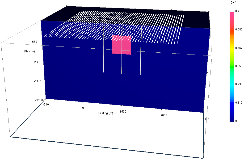
Fig. 5.1 The density model used to generate synthetic data in three vertical boreholes and on the surface (locations shown in white). The anomalous block is 500 m\(^3\) and has a density contrast of 0.7 g/cm\(^3\). First, the surface data alone will inverted. Then, data from the two boreholes outside of the anomalous block will be added to the surface data and modelled and inverted. Finally, data from all three boreholes as well as the surface data will be inverted.

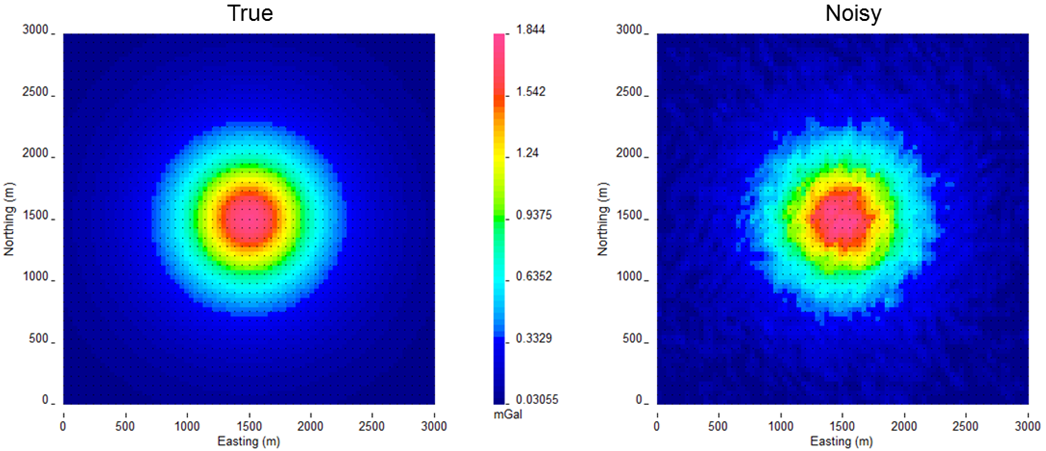
Fig. 5.2 The true data generated by a 500 m\(^3\) block with a density contrast of 0.7 g/cm\(^3\) (left). Gaussian noise with a floor of 0.05 mGal and 2% of the data was added to create the observed data for the inversion (right).

In order run to forward model the surface data, the following was typed into the command line:

gzfor3d mesh.txt loc\_surf.txt model.den

We next simulated the borehole data. The borehole data are calculated in three vertical holes located 500 meters apart (Fig. 5.1) with an interval of 20 meters from 15 to 1,335 m below the surface for a total of 198 data. The command was:

gzfor3d mesh.txt loc\_bh.txt model.den

The borehole dataset has been contaminated with Gaussian noise with a standard deviation of 2% and a floor of 0.01 mGal. The noisy surface data are shown in the right panel of Fig. 5.2. Fig. 5.3 shows the accurate and noisy borehole data. The two datasets are combined to create the “observed” data for the inversion examples in the next section.

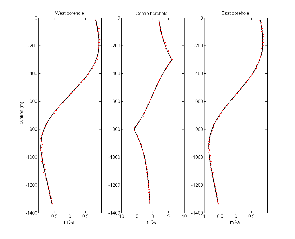
Fig. 5.3 Synthetic borehole data used in the inversions with each panel representing a single borehole. The black lines are true data and red dots are the noisy data.

5.2. Inversion

In this section, we illustrate the inversion of the surface data and then joint inversion of surface and borehole data.

5.2.1. Default parameters

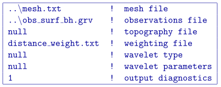
First, the distance weighting function is calculated with PFWEIGHT. Distance weighting was is chosen for consistency between the surface only and surface and borehole inversion solutions (borehole data require distance weighting). The input for the weighting function code is shown below. An example of the created log file is presented in Fig. 5.4.

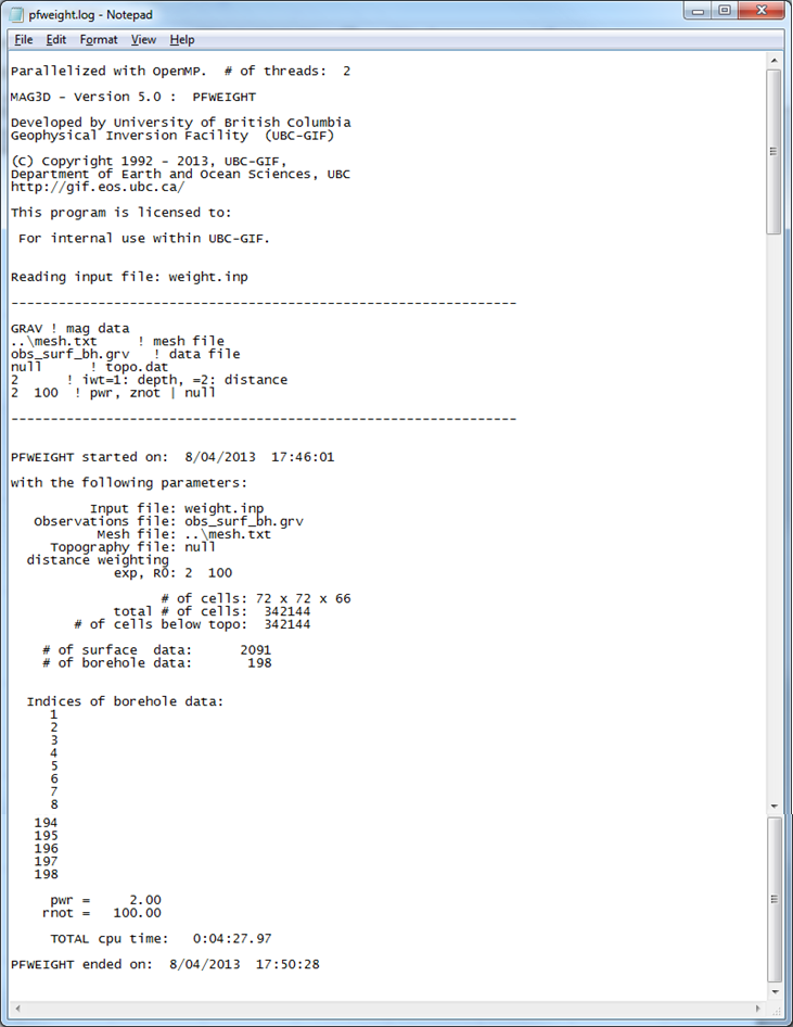
Fig. 5.4 The log file from pfweight. The information within this file reproduces the input file, gives the number of cells in the mesh and below topography, the indices of borehole data within the data file (if applicable), and the time it took for the program to run or any errors that occured.

Next, the sensitivity matrix is calculated with GZSEN3D . The default wavelet compression parameters are used (daub2 with 5% reconstruction error (eps=0.05). We also choose not to output diagnostic parameters, although these are discussed in the Wavelet diagnostic output section. With this scenario chosen, outputs and (these files will be over-written if the program has been run in the same folder more than once without re-naming them). The former file gives the user information about the sensitivity calculation such as compression ratio with the wavelet transform. The latter file will be required during the inversion process. The sensitivity will only have to be re-run if the mesh or data locations are changed. Changing the standard deviations does not require a next .mtx file. The log file from the sensitivity calculation is shown in Fig. 5.5. The input file for the sensitivity calcuation is shown below.

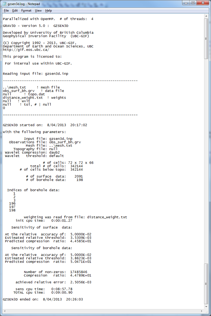
Fig. 5.5 The log file from . The top information gives the input file information and version of the program. The bottom information describes how many cells are in the model after topography, how many data will be inverted, and how well the wavelet transform compressed \(\mathbf{G}\). Typical (and default) wavelet reconstruction error is 5% or eps=0.05 in the input file.

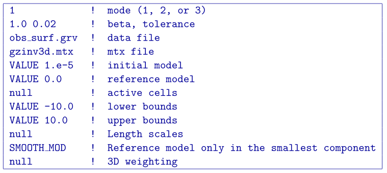
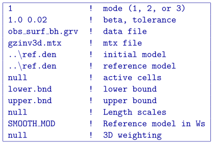
Once the matrix file is created, the inversion can be run by GZINV3D with a general input file. The control file example is provided below. The bounds are set to keep the model between -10 and 10 g/cc (basically creating an “un-bounded” inversion)

The inversion converges in eight iterations. Fig. 5.6 shows the convergence curve for the data misfit versus the iteration number. The desired misfit is approximately 2100 and is achieved within the tolerance given (\(\pm2\%\)). The predicted data from the recovered model is shown on the right of Fig. 5.7 with the observed data on the right for comparison.

An example log file created by GZINV3D within this example set (surface data only) is shown in Fig. 5.8. The file gives the input parameters and general information for every iteration such as the data misfit and iteration CPU time. A developers log (gzinv3d.out) is also written (Fig. 5.9). This file contains detailed information for every iteration including the beta parameter, data misfit, model norm and its components, total objective function, number of conjugate gradient iterations, and the number of truncated cells. The latter is the amount of cells that are at or beyond the bounds and are not included in the minimization with the projected gradient. In this case, it would be cells greater than or equal to 10.0 and less than or equal to -10.0.

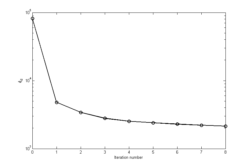
Fig. 5.6 The convergence curve for for the inversion of surface data. The 0\(^{th}\) iteration is the initial misfit. The target misfit is approximately 2,100 where the inversion stops.

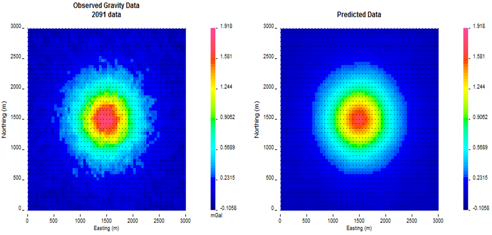
Fig. 5.7 The observed surface data (left) and the surface data created from the recovered model (right). The data are on the same colour scale.

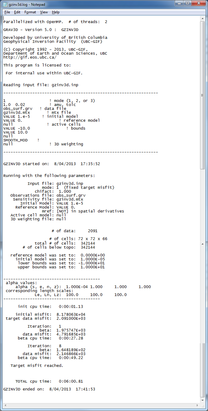
Fig. 5.8 The inversion log created by gzinv3d. As with the sensitivity log file, the top portion of the file gives the input parameters so the results can be reproduced. The bottom gives details for each iteration such as the trade-off parameter, data misfit, and CPU time.

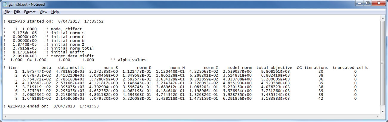
Fig. 5.9 The developer’s log created by gzinv3d. The top portion shows the start time and date and the details of the inversion at each iteration: beta, data misfit, model norm in each direction, total objective function, CG iterations, and the number of truncated cells within the projected gradient routine. The ending data and time is also written to file to be able to match with the simplified log file.

A slice of the recovered model through the centre of the anomalous body is presented in Fig. 5.10 (top). The anomaly has small amplitude and is smoothed. The two boreholes that do not intersect the anomaly are then added. The data are inverted with the same parameters as previous given for the surface-only example and achieves the appropriate data misfit. The recovered model is shown in Fig. 5.10 (middle). The anomalous body is tighter and a bit more constrained with the addition of subsurface data. Finally, the third borehole that intersects the anomaly is added to the observed data. An interesting observation of the recovered model (Fig. 5.10 ; bottom) is the lack of density contrast where the borehole is physically located.

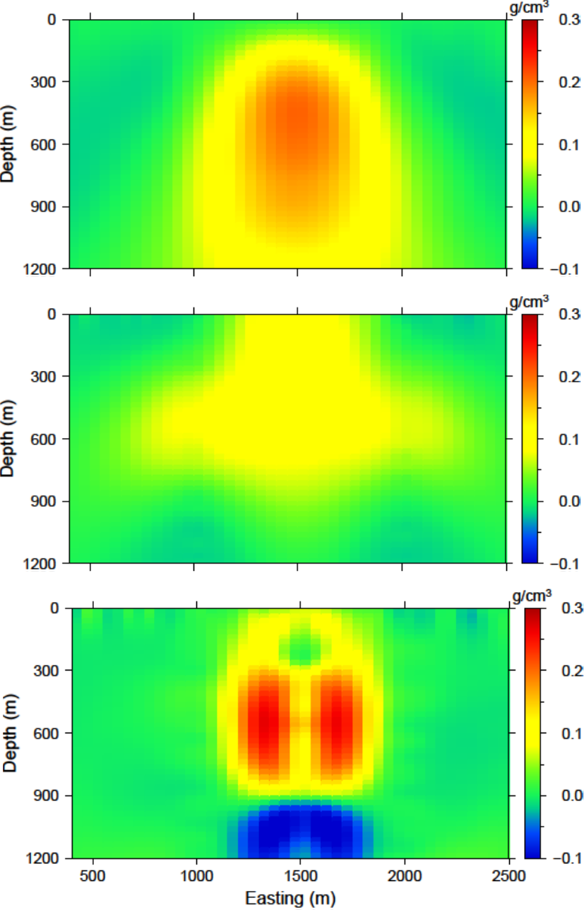
Fig. 5.10 The recovered models from (top) surface only, (middle) surface and the east and west boreholes, and (bottom) surface and three boreholes. The addition of borehole data aids by increasing the amplitude of the recovered anomaly and its compactness. The middle of the anomaly lacks density contrast when the borehole that intersects the anomaly is used. We will further examine ways to alleviate this problem, beginning with the distance weighting parameters.

There are two different types of constraints that can be used in order to recover an anomalous body near the borehole that physically intersects it. Those types are soft or hard constraints. Soft constraints are applied through the model objective function and hard constraints are provided through active and inactive cells, and bounds. The following two sections apply each one of these types of constraints, respectively, in order to alleviate this problem.

5.2.2. Use of soft constraints

One type of constraints that can be used to connect the body for a more realistic interpretation is soft constraints. We examine both the use of distance weighting and the reference model through the model objective function.

5.2.2.1. Distance weighting

Distance weighting is utilized to avoid placing susceptible cells near the observation locations where the mesh has a higher sensitivity and can drive the final solution. We therefore manually change the \(R_o\) (via the distance weighting function) in the input file. We change it from the default value of \(1/4\) of a cell to 100 - much larger than what is needed. Since the values are then normalized, this will allow susceptible material near the borehole locations. The \(\alpha\) value should be 2.0 due to the field decay to a squared power. The sensitivity and inversion input files stay the same. The weighting input file for this example is

The inversion is run with all three boreholes and surface data. A slice of the recovered model is shown in Fig. 5.11. The recovered model has a single anomaly as desired. The anomaly is near the true density contrast (0.7 g/cm\(3\)) and has a block-like shape to it. A by-product of using this weighting is that the algorithm is able to place density not only near the borehole locations, but also near surface observations. To improve upon the results, we examine the use of the reference model with this weighting in order to centralize the anomalous density contrast.

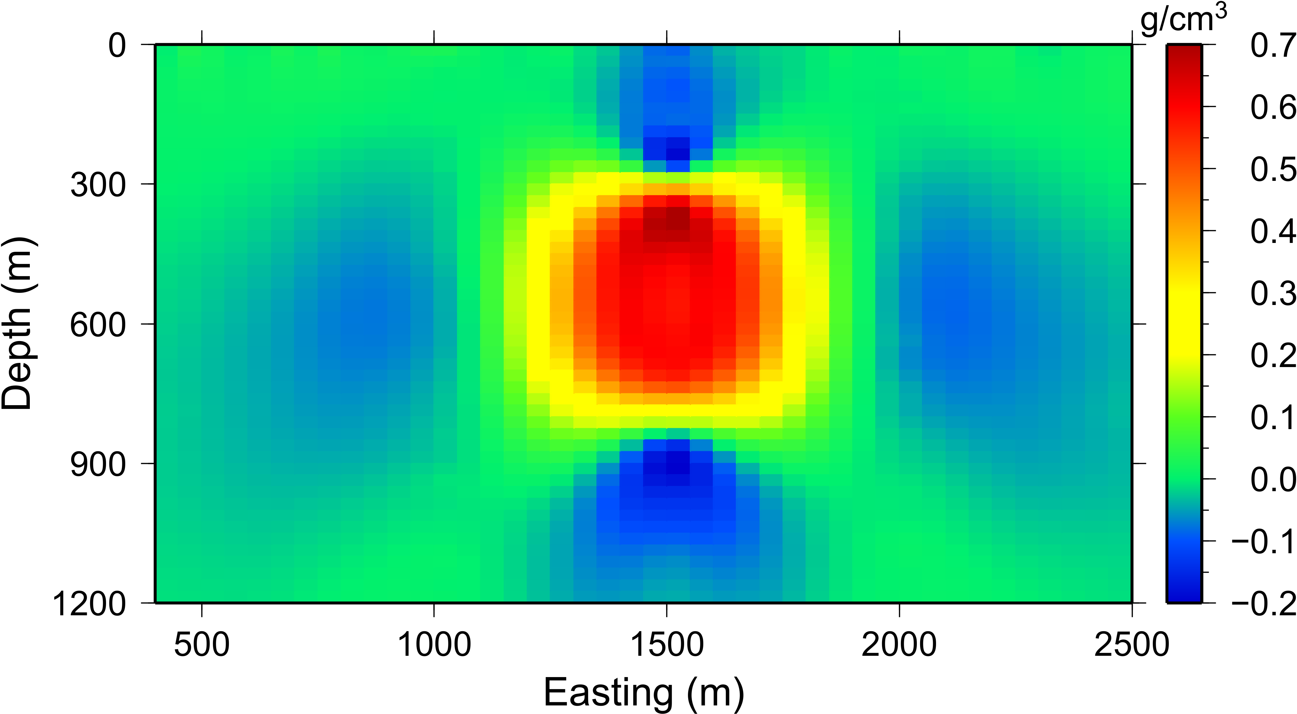
Fig. 5.11 The recovered model after increasing the distance weighting function during the sensitivity calculation. The \(R_o\) was increased to 100. The anomaly is much more compact, although the anomaly reaches the surface to counter-act the strong negative below the true block that is being dictated by the borehole data.

5.2.2.2. Reference model

As previously discussed in the theory section, the reference model can either be incorporated into the spatial derivatives or only the smallest model component of the model objective function. We use the GZSEN3D input file from distance weighting and examine the differences in the recovered model with the addition of the reference model.

The centre borehole intersects the anomaly so we assume that we know the true model at the location of those subsurface observations. The reference model is then designed so that everywhere else it promotes a zero model. A cross section of the reference model is shown in Fig. 5.12 (top). Only the cells that the borehole intersects the anomaly are given as density contrasts above zero.

The input file for the inversion with the reference model throughout model objective function is shown below. The initial model is the same as the reference model and the choice SMOOTH_MOD_DIF is invoked in order to place the reference model in the spatial derivatives.

The recovered model is found in Fig. 5.12 (middle). There is a single anomaly with the maximum amplitude where the non-zero portion of the reference model influenced the solution. The surrounding part of the body goes to zero to try to minimize the difference spatially leaving a strip where the non-zero part of the reference model is located. In this light, the affects of the penalizing the derivatives with the reference model included become apparent.

Next, the input file for the inversion is changed so that the option SMOOTH_MOD is used in order to place the reference model only in the smallest component of the model objective function. A cross section of the recovered model with this option is presented in Fig. 5.12 (bottom). This time the recovered anomaly is much more homogeneous and is closer to the true model throughout the body, although still smaller in amplitude. The solution is similar to just the distance weighting, though it recovers higher density contrasts with a large negative anomaly below.

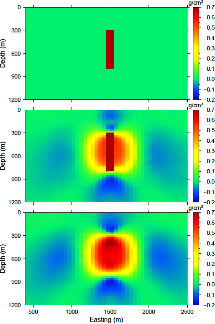
Fig. 5.12 (top) The reference model used from prior information given in the boreholes. The reference model can be utilized (middle) throughout all derivatives of the model objective function or (bottom) just in the smallest model component.

5.2.3. Use of hard constraints

The last section discussed the flexibility of the model objective function to influence the result of GZINV3D. This section examines using hard constraints that strictly enforce a range of values rather than promote the values mathematically. We first incorporate bound constraints and then set key cells to be inactive within inversion.

5.2.3.1. Bounds cells

To be able to appropriate bound the model to reasonable values, we examine the susceptibility given by the borehole information. The bound model file is two columns and requires a lower and upper bound, respectively. For the lower bound, we set the model to zero everywhere but the intersection of the anomaly with the centre borehole. The true model is observed here, so we set the bounds in this region to 0.699 - just below the 0.7 g/cm\(^3\) of the anomalous body (Fig. 5.13 ; top). The upper bounds are 1 everywhere (e.g., positivity based on the borehole) but in the locations of the zero density contrast found in the boreholes. This model can be found in Fig. 5.13 (middle). These two models create the bounds file. We use the same reference model from the soft constraints section. The reference model is is only incorporated in the smallest model component of the model objective function. The input file for the inversion with bounds is

and a cross section of the recovered model is found in Fig. 5.13 (bottom). The bounds force the model to the correct 0.7 g/cm\(^3\) values where the centre borehole intersects the anomalous body, to zero where the boreholes do not intersect any anomalous density, and allows the rest of the model to change as necessary at and above zero. The result is large values in the centre of the anomaly with smoothly decaying amplitudes towards the outsides of the body. The shape is correctly recovered at depth and the large negative anomaly disappears.

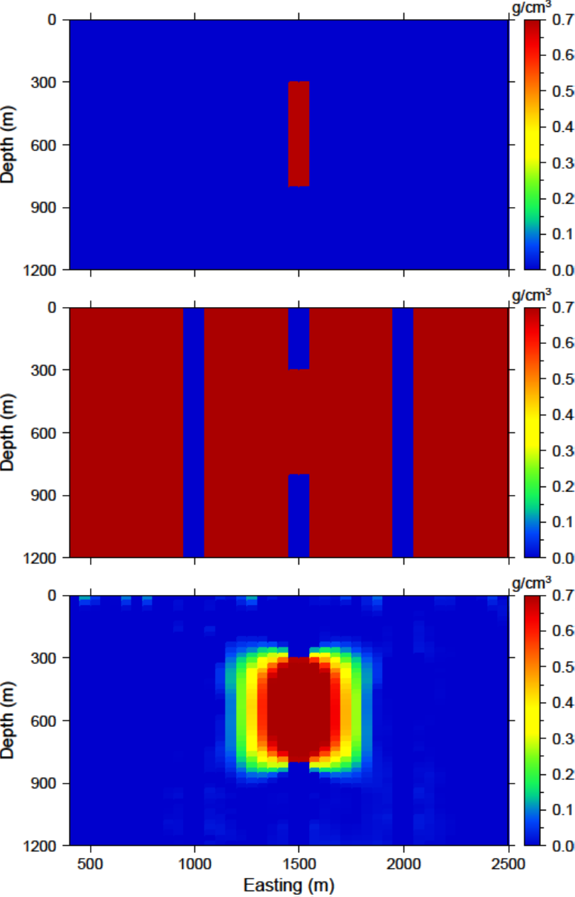
Fig. 5.13 (top) The lower bounds are zero everywhere to enforce positivity, but the intersecting section of the centre borehole. (middle) The upper bounds are 0.0001 g/cm$^3$ where no density contrast was found in the boreholes, 0.701 g/cm$^3$ in the centre borehole where the anomaly is, and 1 g/cm$^3$ everywhere else in the model effectively enforcing only positivity. (bottom) The recovered model with bounds and an initial model.

5.2.3.2. Active/inactive cells

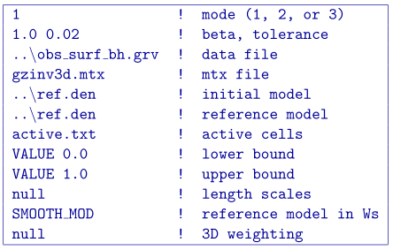
An added functionality of GZINV3D is the ability to set cells to a prescribed value and not incorporated them directly into the inversion. For this example, the model cells in the boreholes are set to inactive. This means they will be stay the value given in the initial model and will not be part of the model objective function (they will contribute to the produced data of the solution). For this example, we set the active cells with values of 1 near the boreholes where the inversion will solve for density contrast. The cells intersecting the boreholes where the density is known is set to \(-1\) in order to influence the model objective function, yet set the cell values. The cells outside the region of interest and that we know have no anomalous density contrast are set to \(0\) (also inactive) and are not included within the inversion. Fig. 5.14 (top) is a cross section of the active cell model. The reference model determines the cell values within the inactive region so the file ref.den is used. For this example, we keep positivity by simply using a lower bound of zero and an upper bound of 1 g/cm\(^3\). An initial model using the reference model is also set. The inversion input file for this example is

The recovered model is shown in Fig. 5.14 (bottom). The centre of the anomaly has the expected value of 0.7 (it was not part of the inversion) and the surrounding density contrast expands to the region of the true anomalous body continuously due to keeping the reference model in the smallest model component of the model objective function. Active cells can improve the inversion when prior information is available.

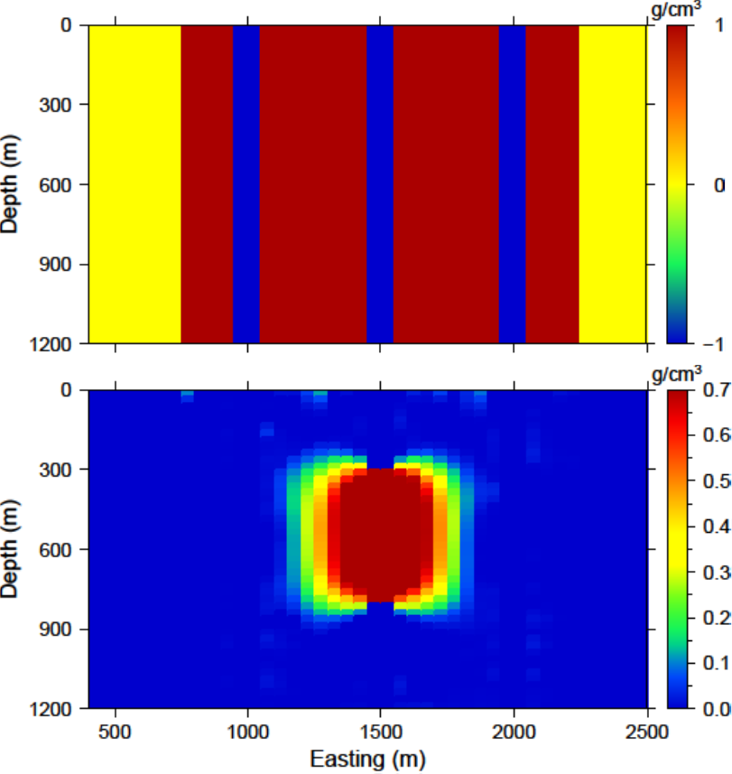
Fig. 5.14 (top) The inactive (-1 and 0) and active (1) cells that are incorporated into the inversion. The reference model sets the values of the inactive cells. The inactive cells set to -1 influence the model objective function. (bottom) A cross section of the recovered model given the inactive cells with the true density values.

5.3. Wavelet diagnostic tests

In this section, we discuss two approaches to try to understand the influence of the wavelet compression onto the recovered model. The diagnostic test output from GZSEN3D is first examined. Then, the combination of GZFOR3D and GZPRE3D is a seldom used, but useful tool in understanding the data affected by the wavelet transform.

5.3.1. Running the diagnostic test tool

In order to run the diagnostic test via GZSEN3D, a 1 is given on the bottom line of the input file. The weighting code and run prior to the sensitivity and the sensitivity matrix output can be used (as if the test was not run) in GZINV3D. It should be noted that the testing can require up to twice the CPU time than running the sensitivity matrix calculation alone. Once the diagnostic testing begins, the user may decide to stop the code. In that case, the testing files are not output yet the matrix file has been written and the inversion process can proceed. An example input file for the sensitivity calculation with testing is

The standard outputs of running are the sensitivity matrix file (gzinv3d.mtx), the average sensitivity for each cell (sensitivity.txt), and the log file (gzsen3d.log). The average sensitivity for each cell is a model file and can be viewed in meshTools3D. The average sensitivity is calculated from the full, non-compressed sensitivity. Running the diagnostic test performs this calculation on the compresses sensitivity and outputs the file sensitivity_compressed.txt. The true compression error is also given in the log file with this setting to be able to compare to the given compression error (e.g., 0.05).

Examining how the two average sensitivity models differ can give insight on how well the wavelet compression has performed. The general shape should be the same, but large jumps in cell size can create large differences, which will be observed with the two outputs. Fig. 5.15 (top) shows a cross-section of the uncompressed sensitivity average for the block example given in this manual. The same cross-section for the compressed average sensitivity for a 5% reconstruction error is presented in Fig. 5.15 (middle). In general, the compression shows good accuracy. The difference between the two models is given in Fig. 5.15 (bottom) for reference. All of the pictures are shown in log scale.

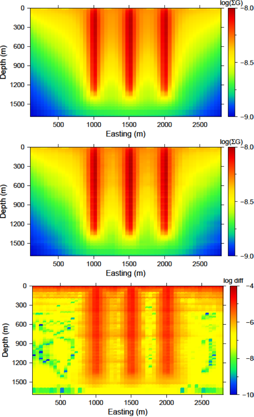
Fig. 5.15 (top) The log of average sensitivity for each cell prior to compression. (middle) the log of average sensitivity for each cell after compression with a 95% reconstruction accuracy. (bottom) The difference between (top) and (middle) on a log scale.

The data from the compressed and uncompressed sensitivity given a constant model of 0.01 is also written, aptly named data_compressed.txt and data_uncompressed.txt respectively. This also gives insight to the differences in column-based integration of the compressed and uncompressed sensitivity matrix. However, the model output is much more intuitive.

5.3.2. Recovered model-based diagnostic test

Users of the this software package often are curious how the wavelet transform is affecting the predicted data. Although the diagnostic test does this calculation on a constant model of 0.1, this test is actually easy to perform once the inversion code has a solution. The gzinv3d_xxx.pre is the predicted data from the compressed sensitivity (for the “xxx” iteration) and can also be calculated with the code GZPRE3D given a file and a recovered model. To obtain the predicted data for an uncompressed sensitivity matrix, run GZFOR3D on the recovered model, gzinv3d_xxx.den. The difference between the generated data sets will show how the wavelet compression is affecting the final data. Large discrepancies in the data may suggest the use of a smaller reconstruction error given on the eps line of the sensitivity input file. An example is shown using the surface-only data set. The two data sets for the uncompressed, compressed sensitivity matrix, and their difference is respectively shown in Fig. 5.16. The maximum difference between the two data sets less than is 0.01 mGal.

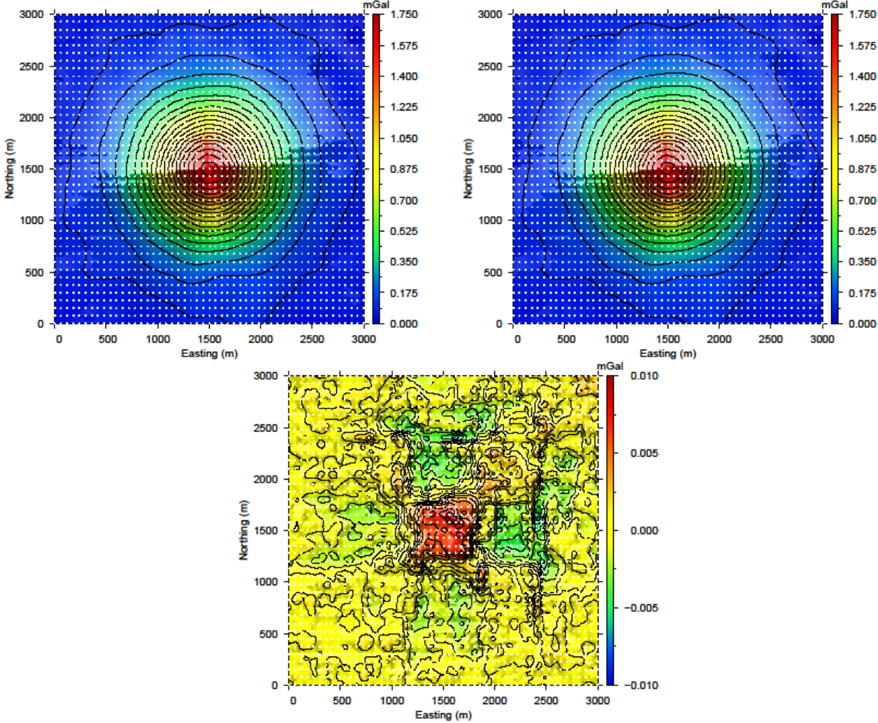
Fig. 5.16 (top-left) The predicted data from the uncompressed sensitivity matrix by using gzfor3d on the recovered model. (top-right) The predicted data from the compressed sensitivity matrix given by gzinv3d or calculated by gzpre3d given the recovered model. (bottom) The difference of the two data sets is less than 0.01 mGal. Data locations are denoted by the white dots.